2 lijsten vergelijken

14 September 2026News around the worldadmin

Oorspronkelijk geplaatst op: 2 oktober 2016

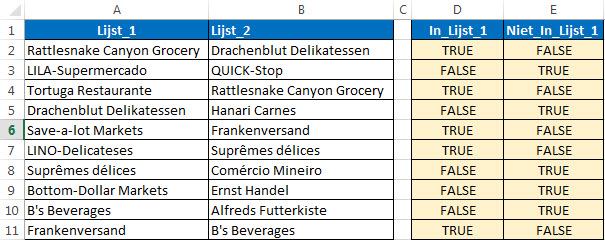
Je kent dat wel. Je hebt twee lijsten die gegevens bevatten. Nu wil je checken of de items in Lijst_2 voorkomen in Lijst_1. Als het lange lijsten zijn is dat een hels karwei.
Bijvoorbeeld, komt “Drachenblut Delikatessen” voor in Lijst_1? Ja (TRUE). Komt “QUICK-Stop” voor in Lijst_1? Nee (FALSE).

Formule die je daarvoor kan gebruiken is simpel:
D1 =ISNUMBER(MATCH($B2;$A$2:$A$11;0))
Doorvoeren naar beneden.

Wil je weten of een item NIET in Lijst_1 voorkomt dan gebruik je de formule:
E1 =ISNA(MATCH($B2;$A$2:$A$11;0))
Doorvoeren naar beneden.

Webscraping gegevens ophalen van een webpagina

14 September 2026Excel and VBAadmin

Oorspronkelijk geplaatst op: 2 oktober 2016

Snel gegevens ophalen van het web ook wel webscraping genoemd. We surfen daarvoor naar:

https://www.autoscout24.de/lst/ford/granada?sort=standard&desc=0&ustate=N%2CU&atype=C&cy=D&ocs_listing=include&source=homepage_search-mask

en willen de prijzen van de old-timer Ford Granada downloaden. Simpel. Onderstaande code kopiëren en in een moduleblad plakken en op F5 slaan. We halen de title en de prijs op.

Lees onderstaande rode gedeelte goed

‘*****************************************************
‘Geef een verwijzing op naar:
‘Microsoft HTML Object Library
‘Te bereiken via: Alt+F11 | Extra | Verwijzingen
‘*****************************************************

Option Explicit

'Tools->Refernces Microsoft HTML Object Library

'MSDN - URLDownloadToFile function - https://msdn.microsoft.com/en-us/library/ms775123(v=vs.85).aspx
Private Declare PtrSafe Function URLDownloadToFile Lib "urlmon" Alias "URLDownloadToFileA" _
(ByVal pCaller      As Long, ByVal szURL As String, ByVal szFileName As String, _
ByVal dwReserved    As Long, ByVal lpfnCB As Long) As Long

Sub Find_Ford_Granada()
    
    Dim fso         As Object
    Set fso = CreateObject("Scripting.FileSystemObject")
    
    Dim sLocalFilename As String
    sLocalFilename = Environ$("TMP") & "\urlmon.html"
    
    Dim sURL        As String
    sURL = "https://www.autoscout24.de/lst/ford/granada?sort=standard&desc=0&ustate=N%2CU&atype=C&cy=D&ocs_listing=include&source=homepage_search-mask"
    
    Dim bOk         As Boolean
    bOk = (URLDownloadToFile(0, sURL, sLocalFilename, 0, 0) = 0)
    If bOk Then
        If fso.FileExists(sLocalFilename) Then
            
            'Tools->References Microsoft HTML Object Library
            Dim oHtml4 As MSHTML.IHTMLDocument4
            Set oHtml4 = New MSHTML.HTMLDocument
            
            Dim oHtml As MSHTML.HTMLDocument
            Set oHtml = Nothing
            
            'IHTMLDocument4.createDocumentFromUrl
            'MSDN - IHTMLDocument4 createDocumentFromUrl method - https://msdn.microsoft.com/en-us/library/aa752523(v=vs.85).aspx
            Set oHtml = oHtml4.createDocumentFromUrl(sLocalFilename, "")
            
            'need to wait a little whilst the document parses
            'because it is multithreaded
            While oHtml.readyState <> "complete"
                DoEvents        'do not comment this out it is required to break into the code if in infinite loop
            Wend
            Debug.Assert oHtml.readyState = "complete"
            
            Dim sTest As String
            sTest = Left$(oHtml.body.outerHTML, 100)
            Debug.Assert Len(Trim(sTest)) > 50        'just testing we got a substantial block of text, feel free to delete
            
            'You can log the information in a textfile. Uncheck the next line.
            'LogInformation (oHtml.body.outerHTML)
            
            'this is where the page specific logic now goes, here I am getting info from Autoscout page
            
            Dim htmlBrand As Object        'MSHTML.DispHTMLElementCollection
            Dim htmlPrice As Object        'MSHTML.DispHTMLElementCollection
            Set htmlBrand = oHtml.getElementsByTagName("h2")
            Set htmlPrice = oHtml.getElementsByClassName("CurrentPrice_price__Ekflz")
            
            Dim lngCounterLoop As Long
            For lngCounterLoop = 0 To htmlBrand.Length - 1
                Dim vBrand
                Dim vPrice
                Set vBrand = htmlBrand.Item(lngCounterLoop)
                Set vPrice = htmlPrice.Item(lngCounterLoop)
                
                'On Error GoTo err_chk
                If vBrand Is Nothing Or vPrice Is Nothing Then
                    Debug.Print "There are no more car brands Or prices To be found Or available"
                Else
                    Debug.Print vBrand.outerText & " - " & vPrice.outerText
                End If
                'On Error GoTo 0
            Next
        End If
    End If
    
    'err_chk:
    '   If Err.Number = 91 Then
    '      MsgBox "There was an ERROR!!! - " & Err.Number & " :  " & Err.Description & vbNewLine & "There are no more brand or price for cars available"
    ' Else
    '    MsgBox Err.Number & ":" & Err.Description
    'End If
End Sub

Option Explicit

'Tools->Refernces Microsoft HTML Object Library

'MSDN - URLDownloadToFile function - https://msdn.microsoft.com/en-us/library/ms775123(v=vs.85).aspx
Private Declare PtrSafe Function URLDownloadToFile Lib "urlmon" Alias "URLDownloadToFileA" _
(ByVal pCaller      As Long, ByVal szURL As String, ByVal szFileName As String, _
ByVal dwReserved    As Long, ByVal lpfnCB As Long) As Long

Sub Find_Ford_Granada()
    
    Dim fso         As Object
    Set fso = CreateObject("Scripting.FileSystemObject")
    
    Dim sLocalFilename As String
    sLocalFilename = Environ$("TMP") & "\urlmon.html"
    
    Dim sURL        As String
    sURL = "https://www.autoscout24.de/lst/ford/granada?sort=standard&desc=0&ustate=N%2CU&atype=C&cy=D&ocs_listing=include&source=homepage_search-mask"
    
    Dim bOk         As Boolean
    bOk = (URLDownloadToFile(0, sURL, sLocalFilename, 0, 0) = 0)
    If bOk Then
        If fso.FileExists(sLocalFilename) Then
            
            'Tools->References Microsoft HTML Object Library
            Dim oHtml4 As MSHTML.IHTMLDocument4
            Set oHtml4 = New MSHTML.HTMLDocument
            
            Dim oHtml As MSHTML.HTMLDocument
            Set oHtml = Nothing
            
            'IHTMLDocument4.createDocumentFromUrl
            'MSDN - IHTMLDocument4 createDocumentFromUrl method - https://msdn.microsoft.com/en-us/library/aa752523(v=vs.85).aspx
            Set oHtml = oHtml4.createDocumentFromUrl(sLocalFilename, "")
            
            'need to wait a little whilst the document parses
            'because it is multithreaded
            While oHtml.readyState <> "complete"
                DoEvents        'do not comment this out it is required to break into the code if in infinite loop
            Wend
            Debug.Assert oHtml.readyState = "complete"
            
            Dim sTest As String
            sTest = Left$(oHtml.body.outerHTML, 100)
            Debug.Assert Len(Trim(sTest)) > 50        'just testing we got a substantial block of text, feel free to delete
            
            'You can log the information in a textfile. Uncheck the next line.
            'LogInformation (oHtml.body.outerHTML)
            
            'this is where the page specific logic now goes, here I am getting info from Autoscout page
            
            Dim htmlBrand As Object        'MSHTML.DispHTMLElementCollection
            Dim htmlPrice As Object        'MSHTML.DispHTMLElementCollection
            Set htmlBrand = oHtml.getElementsByTagName("h2")
            Set htmlPrice = oHtml.getElementsByClassName("CurrentPrice_price__Ekflz")
            
            Dim lngCounterLoop As Long
            For lngCounterLoop = 0 To htmlBrand.Length - 1
                Dim vBrand
                Dim vPrice
                Set vBrand = htmlBrand.Item(lngCounterLoop)
                Set vPrice = htmlPrice.Item(lngCounterLoop)
                
                'On Error GoTo err_chk
                If vBrand Is Nothing Or vPrice Is Nothing Then
                    Debug.Print "There are no more car brands Or prices To be found Or available"
                Else
                    Debug.Print vBrand.outerText & " - " & vPrice.outerText
                End If
                'On Error GoTo 0
            Next
        End If
    End If
    
    'err_chk:
    '   If Err.Number = 91 Then
    '      MsgBox "There was an ERROR!!! - " & Err.Number & " :  " & Err.Description & vbNewLine & "There are no more brand or price for cars available"
    ' Else
    '    MsgBox Err.Number & ":" & Err.Description
    'End If
End Sub

Het resultaat in het zogenaamde immediate window (als je dit window niet ziet, te bereiken via sneltoets Ctrl+G of via View | Immediate window)

Ford Granada 2.8 i V6 Ghia Turnier Klima – SSD- 5.Gang – € 4.890
Ford Granada L – € 7.999
Ford Granada – € 2.500
Ford Granada Dorchester – € 7.999
Ford Granada I Coupé 1.7 V4 nur 67 TKMHU neuH-Zulassung – € 9.450
Ford Granada 2,8i GhiaVOLL-RESTAURIERT – € 18.300
Ford Granada – € 5.290
Ford Granada US Modell 76er Oldtimer H-Kennzeichen 5.0 V8 – € 7.900
Ford Granada GL-GHIA SERVO/SCHIEBEDACH – € 14.900
Ford Granada MK 2 – 2,0 Automatik – erst 78000 Km. – € 7.800
Ford Granada 2.3 Ghia Automatic 2.Hdn. 86 TKM – € 16.500
Ford Granada |H-Kennzeichen|Scheckheft|Klima|AHK – € 9.970
Ford Granada Granada GL / V6 2,0 Motor / 1 HAND – € 4.000
There are no more car brands or prices to be found or available

When you want to log the information in a textfile. Uncheck the next line.
‘LogInformation (oHtml.body.outerHTML)
In the code above and put the code below in the module.

Sub LogInformation(LogMessage As String)

    Dim fileNum As Integer
    Const LogFileName As String = "C:\temp\textfile.html"

    Open "C:\temp\textfile.html" For Output As #1
    Close #1
    MsgBox "Clear complete"

    fileNum = FreeFile                                ' next file number
    Open LogFileName For Append As #fileNum           ' creates the file if it doesn't exist
    Print #fileNum, LogMessage                        ' write information at the end of the text file
    Close #fileNum                                    ' close the file

End Sub

Sub LogInformation(LogMessage As String)

    Dim fileNum As Integer
    Const LogFileName As String = "C:\temp\textfile.html"

    Open "C:\temp\textfile.html" For Output As #1
    Close #1
    MsgBox "Clear complete"

    fileNum = FreeFile                                ' next file number
    Open LogFileName For Append As #fileNum           ' creates the file if it doesn't exist
    Print #fileNum, LogMessage                        ' write information at the end of the text file
    Close #fileNum                                    ' close the file

End Sub

Gegroepeerde gegevens optellen gebaseerd op 5 criteria

14 September 2026News around the worldadmin

Oorspronkelijk geplaatst op: 5 oktober 2016

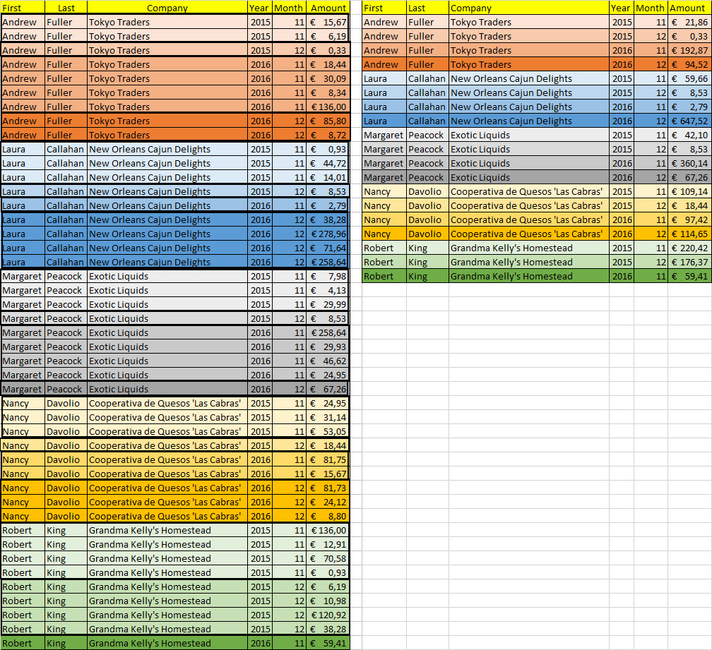
Indien je de bedragen in Kolom F (Amount) wil optellen gebaseerd op de 5 criteria in kolommen A:E (First – Last – Company – Year – Month), heb je wat formules nodig. Vanwege het overzicht zijn de gegevens al gegroepeerd weergegeven. Bekijk bijvoorbeeld de gegevens in Rij 2 en 3. Die zijn hetzelfde namelijk:

Andrew Fuller Tokyo Traders 2015 11
Andrew Fuller Tokyo Traders 2015 11

De twee bedragen bij elkaar opgeteld € 15,67 + € 6,19 = € 21,86
En dat record zie je staan in Rij 2 in de Kolommen H:M

Stel je voor dat de records in Kolommen A:F door elkaar staan en dat het om honderden records gaat, je kunt je dan voorstellen dat het een hele klus is om eerst alles te sorteren en vervolgens de bedragen die bij de passende records horen op te tellen. Door enkele formules in de kolommen H:M te plaatsen.

Samengevat: Tel de bedragen in Kolom F op voor elke unieke combinatie in de Rijen A:E.

Dan nu de formules. Je moet natuurlijk eerst gegevens hebben zoals hierboven. Vervolgens maak je een paar benoemde bereiken. Doe dat als volgt:

– Ga met de cursor in je tabel staan.
– Druk op Ctrl+Shift+F3 Je komt bij: Create names from selection.
– Check > Top row
– En dan OK.

Je hebt nu 5 benoemde bereiken namelijk:

First =Sheet2!$A$2:$A$45
Last =Sheet2!$B$2:$B$45
Company =Sheet2!$C$2:$C$45
Year =Sheet2!$D$2:$D$45
Month =Sheet2!$E$2:$E$45

Let op dat de formule naar Sheet2! verwijst.

Vervolgens, ga naar Formulas > Name manager > New. Vul in:
Name: RowVector
Refers to: =ROW(First)-ROW(INDEX(First;1;1))+1

Onderstaande formules invoeren met Ctrl+Shift+Enter

Invoegen met alleen Enter
M2 =IF($H2=””;””;SUMIFS(Amount;First;$H2;Last;$I2;Company;$J2;Year;$K2;Month;$L2))

Alle formules tenslotte doorvoeren naar beneden.

Unieke lijst genereren

14 September 2026News around the worldadmin

Oorspronkelijk geplaatst op: 6 oktober 2016

Een dynamische lijst maken. Dit betekent dat, naar mate je de lijst uitbreidt en dus langer maakt, de lijst zich als het ware aanpast.

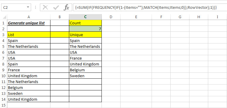
We hebben namen van landen in Kolom A. Sommige landen staan er dubbel in of zelfs driedubbel. In Kolom C willen we slechts unieke namen van landen.

Aan de slag. Zorg dat je gegevens hebt zoals in de afbeelding. Vervolgens dien je een aantal namen met daaraan gekoppeld formules te maken. Doe dat zoals hieronder beschreven:

Formulas > Name manager > New
Name: = RowVector
Refers to: =ROW(Items)-ROW(INDEX(Items;1;1))+1
Klik: OK

Formulas > Name manager > New
Name: = Items
Refers to: =Sheet1!$A$4:INDEX(Sheet1!$A$4:$A$20;Lrow)
Klik: OK

Formulas > Name manager > New
Name: = Lrow
Refers to: =MATCH(REPT(“z”;255);Sheet1!$A$4:$A$20)
Klik: OK

Tenslotte formules in de volgende cellen zetten:

Formule in C2

=SUM(IF(FREQUENCY(IF(1-(Items="");MATCH(Items;Items;0));RowVector);1))

Invoegen met Ctrl+Shift+Enter
Doorvoeren naar beneden.

Formule in C4

=IF(ROWS($C$4:C4)<=$C$2;INDEX(Items;SMALL(IF(FREQUENCY(IF(1-(Items="");MATCH(Items;Items;0));RowVector);RowVector);ROWS($C$4:C4)));"")

Invoegen met Ctrl+Shift+Enter
Doorvoeren naar beneden.

Totalen berekenen, 2 criteria

14 September 2026News around the worldadmin

Oorspronkelijk geplaatst op: 6 oktober 2016

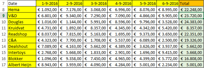
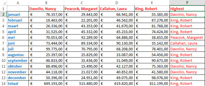
Een paar winkels (Kolom A) hebben goede (of slechte) zaken gedaan en je ziet de resultaten per dag (Kolommen B:G in de afbeelding. De opgave dit keer is om de totalen (Kolom F) te berekenen. Er zijn 2 criteria namelijk, bedrag >= €5000 en de datum moet liggen tussen 2-9-2016 en 5-9-2016.

Formule in H8
=SUMIFS(B8:G8;$B$7:$G$7;”>=”&DATE(2016;9;2);$B$7:$G$7;”<=”&DATE(2016;9;5);B8:G8;”>”&5000)

Doorvoeren naar beneden.

Wie heeft het meest verkocht per maand/jaar

14 September 2026News around the worldadmin

Oorspronkelijk geplaatst op: 8 november 2016

De vertegenwoordigers hebben weer eens goed hun best gedaan maar wie heeft het meeste verkocht per maand en wie is de topverkoper van het jaar?

Formule invoeren met Ctrl+Shift+Enter

Formule in F2

=IFERROR(INDEX($B$1:$E$1;SMALL(IF($B2:$E2=MAX($B2:$E2);COLUMN($B$1:$E$1)-COLUMN($B$1)+1);COLUMNS($F2:F2)));””)

Naar beneden doorvoeren.

Bestanden in map tonen met hyperlinks

14 September 2026News around the worldadmin

Oorspronkelijk geplaatst op: 20 augustus 2019

De VBA code genereert een lijst met bestanden in een map. Je kunt zelf een map (directory) kiezen waarvan je de bestanden wil zien

Option Compare Text
Option Explicit

Function Excludes(Ext As String) As Boolean
Dim X, NumPos As Long
    'Function purpose:  To exclude listed file extensions from hyperlink listing
    
    'Enter/adjust file extensions to EXCLUDE from listing here:
    X = Array("exe", "bat", "dll", "zip")
    
    On Error Resume Next
    NumPos = Application.WorksheetFunction.Match(Ext, X, 0)
    If NumPos > 0 Then Excludes = True
    On Error GoTo 0
End Function

Sub HyperlinkFileList()
'Macro purpose:  To create a hyperlinked list of all files in a user
'specified directory, including file size and date last modified
'NOTE:  The 'TextToDisplay' property (of the Hyperlink object) was added
'in Excel 2000.  This code tests the Excel version and does not use the
'Texttodisplay property if using XL 97.

Dim fso As Object, ShellApp As Object, File As Object
Dim SubFolder As Object, Directory As String
Dim Problem As Boolean, ExcelVer As Integer

    'Turn off screen flashing
    Application.ScreenUpdating = False

    'Create objects to get a listing of all files in the directory
    Set fso = CreateObject("Scripting.FileSystemObject")

    'Prompt user to select a directory
    Do
        Problem = False
        Set ShellApp = _
            CreateObject("Shell.Application").Browseforfolder(0, _
            "Please choose a folder", 0, "c:\\")
        On Error Resume Next
        
        'Evaluate if directory is valid
        Directory = ShellApp.self.path
        Set SubFolder = fso.GetFolder(Directory).Files
        If Err.Number <> 0 Then
            If MsgBox("You did not choose a valid directory!" _
                & vbCrLf & "Would you like to try again?", _
                vbYesNoCancel, "Directory Required") <> vbYes Then _
                Exit Sub
            Problem = True
        End If
        On Error GoTo 0
    Loop Until Problem = False

    'Set up the headers on the worksheet
    With ActiveSheet
        With .Range("A1")
            .Value = "Listing of all files in:"
            .ColumnWidth = 40
            
            'If Excel 2000 or greater, add hyperlink with file name
            'displayed.  If earlier, add hyperlink with full path displayed
            
            'Using XL2000+
            If Val(Application.Version) > 8 Then
                .Parent.Hyperlinks.Add Anchor:=.Offset(0, 1), _
                    Address:=Directory, TextToDisplay:=Directory
            
            'Using XL97
            Else
                .Parent.Hyperlinks.Add Anchor:=.Offset(0, 1), _
                    Address:=Directory
            End If
        End With
        With .Range("A2")
            .Value = "File Name"
            .Interior.ColorIndex = 15
            With .Offset(0, 1)
                .ColumnWidth = 15
                .Value = "Date Modified"
                .Interior.ColorIndex = 15
                .HorizontalAlignment = xlCenter
            End With
            With .Offset(0, 2)
                .ColumnWidth = 15
                .Value = "File Size (Kb)"
                .Interior.ColorIndex = 15
                .HorizontalAlignment = xlCenter
            End With
        End With
    End With

    'Adds each file, details and hyperlinks to the list
    For Each File In SubFolder
        If Not Excludes(Right(File.path, 3)) = True Then
            With ActiveSheet
                
                'If Excel 2000 or greater, add hyperlink with file name
                'displayed.  If earlier, add hyperlink with full path displayed
                
                'Using XL2000+
                If Val(Application.Version) > 8 Then
                    .Hyperlinks.Add _
                        Anchor:=ActiveSheet.Range("A65536").End(xlUp).Offset(1, _
                        0), Address:=File.path, _
                        TextToDisplay:=File.Name
                
                'Using XL97
                Else
                    .Hyperlinks.Add _
                        Anchor:=ActiveSheet.Range("A65536").End(xlUp).Offset(1, _
                        0), Address:=File.path
                End If
                
                'Add date last modified, and size in KB
                With .Range("A65536").End(xlUp)
                    .Offset(0, 1) = File.datelastModified
                    With .Offset(0, 2)
                        .Value = _
                            WorksheetFunction.Round(File.Size / _
                            1024, 1)
                        .NumberFormat = "#,##0.0"
                    End With
                End With
            End With
        End If
    Next
End Sub

Unieke lijst genereren

14 September 2026News around the worldadmin

Oorspronkelijk geplaatst op: 27 augustus 2019

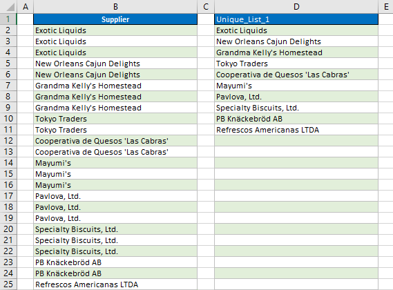
Indien je een unieke lijst wil genereren is dit de manier om dat te doen. De waarden staan in kolom B. Daar staan ook dubbele of zelfs drie-dubbele waarden in:

In D2 zet je de volgende formule:

=IFERROR(INDEX($B$2:$B$1000;SMALL(IF(FREQUENCY(IF($B$2:$B$1000<>””;MATCH($B$2:$B$1000;$B$2:$B$1000;0));ROW($B$2:$B$1000)-ROW(INDEX($B$2:$B$1000;1;1))+1);ROW($B$2:$B$1000)-ROW(INDEX($B$2:$B$1000;1;1))+1);ROWS($A$2:A2)));””)

Dit is een zogenaamde array formule, invoeren met: Ctrl+Shift+Enter, NIET alleen Enter. Als je dit goed hebt gedaan, plaatst Excel accolades om de formule { }.

Let op: Plaats die accolades { } niet handmatig.
Doorvoeren naar beneden.

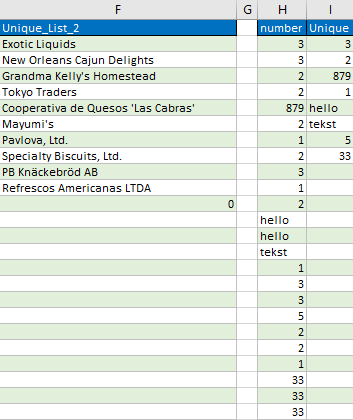
Nog een mogelijkheid met een kortere maar minder robuuste formule

In F2 zet je de volgende formule:
=IFERROR(INDEX($B$2:$B$1000; MATCH(0;COUNTIF($F$1:F1; $B$2:$B$1000);0));””)

Ook dit is weer een array formule, dus invoeren met: Ctrl+Shift+Enter
Doorvoeren naar beneden.

Tenslotte, in kolom H staan tekst en cijfers door elkaar. In kolom I zet je alweer een array formule:

=IFERROR(INDEX($H$2:$H$30;SMALL(IF(FREQUENCY(IF($H$2:$H$30<>””;MATCH($H$2:$H$30;$H$2:$H$30;0));ROW($H$2:$H$30)-ROW(INDEX($H$2:$H$30;1;1))+1);ROW($H$2:$H$30)-ROW(INDEX($H$2:$H$30;1;1))+1);ROWS($A$2:A2)));””)

Ook dit is weer een array formule, dus invoeren met: Ctrl+Shift+Enter
Doorvoeren naar beneden.

Unieke waarden met twee criteria

14 September 2026News around the worldadmin

Oorspronkelijk geplaatst op: 28 augustus 2019

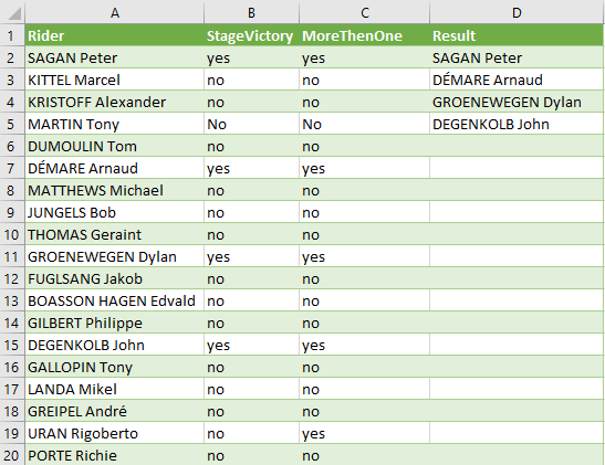
De wielrenners in de Tour de France hebben weer goed hun best gedaan. Sommige renners hebben een etappe gewonnen maar andere renners hebben meer dan 1 etappe gewonnen. Welke renners zijn dat? Ze staan in kolom D. Hiervoor is een ingewikkelde formule gebruikt en die plaats je in D2:

=IFERROR(INDEX($A$2:$A$20;SMALL(IF(FREQUENCY(IF($A$2:$A$20<>””;IF($B$2:$B$20=”yes”;IF($C$2:$C$20=”yes”;MATCH($A$2:$A$20;$A$2:$A$20;0))));ROW($A$2:$A$20)-ROW(INDEX($A$2:$A$20;1;1))+1);ROW($A$2:$A$20)-ROW(INDEX($A$2:$A$20;1;1))+1);ROWS($1:1)));””)

Dit is een zogenaamde array formule, invoeren met: Ctrl+Shift+Enter, NIET alleen Enter. Als je dit goed hebt gedaan, plaatst Excel accolades om de formule { }.

Let op: Plaats die accolades { } niet handmatig.
Doorvoeren naar beneden.

Waarden optellen terwijl Id telkens verandert

14 September 2026News around the worldadmin

Oorspronkelijk geplaatst op: 1 september 2019

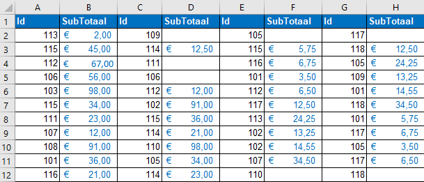
Best een moeilijke klus. In de kolommen A, C, E, G staan de Id’s van de verkopers. In de kolommen B, D, F, H staan de verkoopcijfers. Je wil de verkoopcijfers van elke Id (verkoper) optellen. Natuurlijk is er een probleem, de Id’s en verkoopcijfers kunnen telkens veranderen.

Ten eerste voeg je onderstaande code toe:

1. Kopieer de onderstaande code middels Ctrl + C
2. Druk op de toetscombinatie ALT + F11 om de Visual Basic Editor te openen
3. Druk op de toetscombinatie ALT + N om het menu Invoegen te openen
4. Druk op M om een standaard module in te voegen
5. Daar waar de cursor knippert voeg je de code in middels Ctrl + V

Function ArrayUnion(ParamArray Arg() As Variant) As Variant
' Code: Juan Pablo González
' Spec: Aladin Akyurek
' May 4, 2003
' Ref: TinyURL.com - shorten that long URL into a tiny URL
Dim TempUnion() As Variant
Dim i As Long, Itm As Variant, Ctr As Long
    For i = LBound(Arg) To UBound(Arg)
        Arg(i) = Arg(i)
        If IsArray(Arg(i)) Then
            For Each Itm In Arg(i)
                Ctr = Ctr + 1
                ReDim Preserve TempUnion(1 To Ctr) As Variant
                TempUnion(Ctr) = Itm
            Next Itm
        Else
            Ctr = Ctr + 1
            ReDim Preserve TempUnion(1 To Ctr) As Variant
            TempUnion(Ctr) = Arg(i)
        End If
    Next i
ArrayUnion = TempUnion
End Function

Vervolgens heb je de volgende formules nodig. Eerst maak je 2 benoemde bereiken. Ga naar:

Formulas | Name manager | New

en geef de naam Ivec. Vervolgens:

In het vak Refers to zet je de volgende formule:

=ROW(INDIRECT(“1:”&COLUMNS(PNdata)))

Herhaal dit:
Naam: PNdata
Refers to:
=arrayunion(Sheet1!$A$2:$A$12;Sheet1!$C$2:$C$12;Sheet1!$E$2:$E$12;Sheet1!$G$2:$G$12)

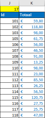
In J1: =SUM(IF(FREQUENCY(IF(PNdata<>””;MATCH(“~”&PNdata;PNdata&””;0));Ivec);1))

Dit is een zogenaamde array formule, invoeren met: Ctrl+Shift+Enter, NIET alleen Enter. Als je dit goed hebt gedaan, plaatst Excel accolades om de formule { }. Let op: Plaats die accolades { } niet handmatig.

In J3:
=IF(ROWS($J$3:J3)<=$J$1;MIN(IF(ISNUMBER(MATCH(PNdata;$J$2:J2;0));””;PNdata));””)
Doorvoeren naar beneden.

Dit is een zogenaamde array formule, invoeren met: Ctrl+Shift+Enter, NIET alleen Enter. Als je dit goed hebt gedaan, plaatst Excel accolades om de formule { }. Let op: Plaats die accolades { } niet handmatig.

In K3: =SUMIFS(B:H;A:G;J3)
(Dit is GEEN array formule, dus gewoon invoeren met alleen Enter).
Doorvoeren naar beneden.

Afbeelding 1

Afbeelding 2

Credits gaan naar:
Code: Juan Pablo González
Spec: Aladin Akyurek
Source: https://tinyurl.com/y3b9r9qg
May 4, 2003