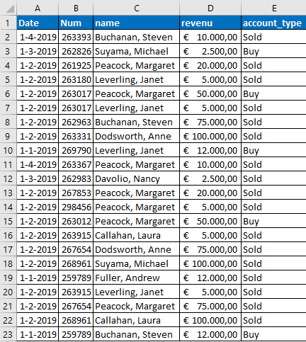
On Sheet1 the names of sellers are in Column C and in Column D are amounts. In Column C, the name of the same employee can appear multiple times.

On Sheet2, we want to show the seller with the highest total amount and then the second seller, etc. A kind of Top 10 so to speak. In addition, there is a criterion, we only count the amounts for which column E says “Sold”.

Sheet1

Sheet2

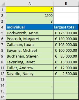
A1 Since you want to see a Top-N, enter the number here, for example 8. Then you get to see the Top-8.

You have to enter the formulas with Ctrl+Shift+Enter (not just Enter)

A2 =LARGE(SUMIFS(Sheet1!$D$2:$D$23;Sheet1!$C$2:$C$23;IF(FREQUENCY(IF(1-(Sheet1!$C$2:$C$23="");MATCH(Sheet1!$C$2:$C$23;Sheet1!$C$2:$C$23;0));ROW(Sheet1!$C$2:$C$23)-ROW(Sheet1!$C$2)+1);Sheet1!$C$2:$C$23);Sheet1!$E$2:$E$23;"Sold");MIN(A1;SUM(IF(FREQUENCY(IF(1-(Sheet1!$C$2:$C$23="");MATCH(Sheet1!$C$2:$C$23;Sheet1!$C$2:$C$23;0));ROW(Sheet1!$C$2:$C$23)-ROW(Sheet1!$C$2)+1);1))))

A3 =IFERROR(SUM(IF(SUMIFS(Sheet1!$D$2:$D$23;Sheet1!$C$2:$C$23;IF(FREQUENCY(IF(1-(Sheet1!$C$2:$C$23="");MATCH(Sheet1!$C$2:$C$23;Sheet1!$C$2:$C$23;0));ROW(Sheet1!$C$2:$C$23)-ROW(Sheet1!$C$2)+1);Sheet1!$C$2:$C$23))>=A2;1));0)

A5 =IF($B5="";"";INDEX(Sheet1!$C$2:$C$23;SMALL(IF(SUMIFS(Sheet1!$D$2:$D$23;Sheet1!$C$2:$C$23;IF(FREQUENCY(IF(1-(Sheet1!$C$2:$C$23="");MATCH(Sheet1!$C$2:$C$23;Sheet1!$C$2:$C$23;0));ROW(Sheet1!$C$2:$C$23)-ROW(Sheet1!$C$2)+1);Sheet1!$C$2:$C$23);Sheet1!$E$2:$E$23;"Sold")=$B5;ROW(Sheet1!$C$2:$C$23)-ROW(Sheet1!$C$2)+1);COUNTIFS($B$5:B5;B5))))

B5 =IF(ROWS($B$5:B5)>$A$3;"";LARGE(SUMIFS(Sheet1!$D$2:$D$23;Sheet1!$C$2:$C$23;IF(FREQUENCY(IF(1-(Sheet1!$C$2:$C$23="");MATCH(Sheet1!$C$2:$C$23;Sheet1!$C$2:$C$23;0));ROW(Sheet1!$C$2:$C$23)-ROW(Sheet1!$C$2)+1);Sheet1!$C$2:$C$23);Sheet1!$E$2:$E$23;"Sold");ROWS($B$5:B5)))