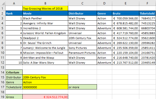
Anders dan de naam doet vermoeden gaan we bij het gebruik van SUMPRODUCT eerst vermenigvuldigen en dan pas optellen. Hieronder vind je een lijst met films uit 2018 en wat bijzonderheden in de diverse kolommen. We willen a.d.h.v. een aantal criteria de juiste resultaten filteren en de bruto inkomsten berekenen. Criteria zijn:
– De distributor is 20th Century Fox
– Genre is Action
– TicketsSold is meer dan 30.000.000 (30 miljoen)

In het bereik B15:B17 plaatsen we de criteria en in B19 komt de formule.

Formule:

In [B19] =SUMPRODUCT(($C$3:$C$12=$B$15)*($D$3:$D$12=$B$16)*($F$3:$F$12>$B$17)*$E$3:$E$12)

Dit resulteert in een reeks TRUE en FALSE:

{FALSE;FALSE;FALSE;FALSE;TRUE;FALSE;FALSE;FALSE;FALSE;FALSE}
{TRUE;TRUE;FALSE;TRUE;TRUE;FALSE;FALSE;TRUE;TRUE;FALSE}
{TRUE;TRUE;TRUE;TRUE;TRUE;FALSE;FALSE;FALSE;FALSE;FALSE}

zoals je weet resulteert:
TRUE in 1
en
FALSE in 0

En dan krijg je:
{0;0;0;0;1;0;0;0;0;0}
{1;1;0;1;1;0;0;1;1;0}
{1;1;1;1;1;0;0;0;0;0}

Dan gaan we vermenigvuldigen. Je ziet dat er maar 1 combinatie is met drie enen (1*1*1) = 1 (rode gedeelte) en die correspondeert met de 5e waarde namelijk 324512774 en dat is tegelijk het eindresultaat omdat we geen verdere waarden hoeven op te tellen.

{700059566;678815482;608581744;417719760;324512774;269622130;235506359;220159104;216648740;213767512}

Verander je de Distributor in Walt Disney dan krijg je:
{1;1;0;0;0;0;0;0;1;1}
{1;1;0;1;1;0;0;1;1;0}
{1;1;1;1;1;0;0;0;0;0}

We gaan weer eerst vermenigvuldigen. Je ziet dat er nu 2 combinatie zijn met drie enen (1*1*1) = 1 (rode gedeelte) en die corresponderen met de 1e waarde en 2e waarde. Die tellen we op en krijgen als resultaat 1.378.875.048

{700059566;678815482;608581744;417719760;324512774;269622130;235506359;220159104;216648740;213767512}

Als je met Visual Basic for Applications werkt, kun je verwijzingen instellen naar andere, zogenaamde, bibliotheken. Dit zijn geen boeken maar een soort van kleine programma’s. Indien je nog niet in de Visual Basic Editor bent, druk je op Alt+F11.
Vervolgens op Tools | References. Je krijgt dan een menu waarin je talloze bibliotheken ziet zoals:

– Microsoft Scripting Runtime
– Microsoft Internet Controls
– Microsoft HTML Object Library
– Microsoft XLM, v6.0

Hoe vaak komt een woord voor in een tekst? Ik zou niet weten waarom je dat zou willen weten. Maar met Excel kun je zoiets berekenen.
In afbeelding 1 zie je in Cel A1 en A2 een paar zinnen uit de welbekende  Lorem Ipsum tekst.

AFBEELDING 1

In Afbeelding 2 zie je een gedeelte van het resultaat.

AFBEELDING 2

De VBA code die je kunt gebruiken.
LET OP, de eerste code is hoofdletter gevoelig. Dat betekent dat bijvoorbeeld het woord “nulla” anders is als het woord “Nulla”. Beide woorden komen daarom 2x voor.

Option Explicit

Sub Hoe_Vaak_Komt_Dat_Woord_Voor()
'Zet Data in meerdere cellen van Kolom A.
'Data alleen in A1 geeft foutmelding
'Data in Kolom A, resultaat komt in de Kolommen C:D.

Dim x As Long, Cnt As Long, Txt As String, Arr() As String
    Txt = " " & Join(Application.Transpose(Range([A1], Cells(Rows.Count, "A").End(xlUp)))) & " "
    
    For x = 2 To Len(Txt)
        If Mid(Txt, x, 1) = "'" And Not Mid(Txt, x - 1, 3) Like "[A-Za-z0-9]'[A-Za-z0-9]" Then
            Mid(Txt, x) = " "
        ElseIf Mid(Txt, x, 1) Like "[!A-Za-z0-9']" Then
            Mid(Txt, x) = " "
        End If
    Next
    
    Arr = Split(Application.Trim(Txt))
    
    With CreateObject("scripting.dictionary")
        
        For x = 0 To UBound(Arr)
            .Item(Arr(x)) = .Item(Arr(x)) + 1
        Next
        
        Cnt = .Count
        Range("C2").Resize(Cnt) = Application.Transpose(.Keys)
        Range("D2").Resize(Cnt) = Application.Transpose(.items)
    End With
    
    Range("C2:D" & Cnt).Sort Range("C2"), xlAscending, Range("D2"), , xlDescending, Header:=xlNo, MatchCase:=False
End Sub

LET OP, de tweede code is NIET hoofdletter gevoelig. Dat betekent dat bijvoorbeeld het woord “nulla” hetzelfde is als het woord “Nulla” en daarom 4x voor komt.

Sub Hoe_Vaak_Komt_Dat_Woord_Voor_Met_RegExp()
'Data in Kolom A, resultaat komt in de Kolommen F:G.
'*****************************************************
'Geef een verwijzing op naar:
'Microsoft Forms 2.0 Object Library
'Te bereiken via: Alt+F11 | Tools | References
'*****************************************************

Dim regEx As Object, matches As Object, x As Object, d As Object
Dim obj As New DataObject
Dim tx As String, z As String

    Range("A1", Cells(Rows.Count, "A").End(xlUp)).Copy
    obj.GetFromClipboard
    tx = obj.GetText
    Application.CutCopyMode = False
    tx = Replace(tx, "'", "___")
        
    Set regEx = CreateObject("VBScript.RegExp")
    
    With regEx
        .Global = True
        .MultiLine = True
        .IgnoreCase = True
        .Pattern = "\w+"
    End With
    
    Set d = CreateObject("scripting.dictionary")
    d.CompareMode = vbTextCompare
        
    Set matches = regEx.Execute(tx)
            
        For Each x In matches
            z = CStr(x)
            If Not d.Exists(z) Then
                d(z) = 1
            Else
                d(z) = d(z) + 1
            End If
        Next
                    
    If d.Count = 0 Then MsgBox "Nothing found": Exit Sub
    Range("D:E").ClearContents
    
    'put the result in col D:E
        With Range("F2").Resize(d.Count, 2)
            .Cells = Application.Transpose(Array(d.Keys, d.items))
            .Replace What:="___", Replacement:="'", LookAt:=xlPart, SearchFormat:=False, ReplaceFormat:=False
        End With
    'Sort
    Range("F2:G" & d.Count).Sort Range("F2"), xlAscending, Range("G2"), , xlDescending, Header:=xlNo, MatchCase:=False
End Sub

In Kolom A staan bedrijven. Sommige bedrijven staan er meerdere keren in. We hebben dus te maken met dubbele waarden in kolom A

We willen in dit voorbeeld de HOOGSTE waarde van Hasbro, Inc.
In D2 kun je een validatielijst maken met alle namen van de bedrijven zodat je gemakkelijk een bedrijf kunt selecteren.

Om dat te doen maak je ergens op je werkblad eerst een unieke lijst met alle bedrijven, Bijvoorbeeld in F2:F14.

Data | Data validation | Data validation | Allow > List | Source > en verwijs naar F2:F14

In [D5] =MAX(INDEX((A2:A21=D2)*B2:B21;0))

Alle hyperlinks op je werkblad verwijderen. Selecteer het bereik met links en zet de code aan het werk.

Sub DeleteHyperlinks()
    With Selection
        .Hyperlinks.Delete
    End With
End Sub

Deze code verwijdert zonder pardon ALLE hyperlinks op je actieve blad.

Sub NoLinks()
    ActiveSheet.Hyperlinks.Delete
End Sub

En deze verwijdert zonder te vragen ALLE afbeeldingen.

Sub NoPictures()
    ActiveSheet.Pictures.Delete
End Sub

Deze werkt iets anders maar verwijdert toch ALLE vormen op het actieve blad.

Sub NoShapes()
    ActiveSheet.Shapes.SelectAll
    Selection.Delete
End Sub

Vul een vierkant met het alfabet waarbij de regels telkens verspringen. In verkorte vorm:

ABCD
BCDA
CDAB
DABC

Maar dan met alle 26 letters.

Sub Fill_Square_With_Alfabet()
Dim strAlfabet As String
Dim Arr(1 To 26, 1 To 26) As Variant

    strAlfabet = "ZABCDEFGHIJKLMNOPQRSTUVWXY"

    For intRow = 1 To 26
        strCharacter = Left(strAlfabet, 1)
        strAlfabet = Mid(strAlfabet, 2, 25) & strCharacter
        For intColumn = 1 To 26
            Arr(intRow, intColumn) = Mid(strAlfabet, intColumn, 1)
        Next
    Next



    For intRow = 1 To 26
        For intColumn = 1 To 26
            Cells(intRow, intColumn).Value = Arr(intRow, intColumn)
        Next
    Next
    
MsgBox "Square created"
End Sub

Function findInverse(m As Integer, modulus As Integer) As Variant
    Dim i As Integer
    Dim xOne As Integer
    Dim xTwo As Integer
    Dim temp As Integer
    Dim remainder As Integer
    Dim divisor As Integer
    Dim dividend As Integer
    Dim allQuotients() As Integer
    
    '-----Calculate the GCD and quotients
    'The expression a = b * q + r will become
    'dividand = divisor * q + remainder
    
    dividend = m
    divisor = modulus

    'need to swap for this one because the number of quotients matters;
    'if a < b then we get a large initial quotient as an extra step
    If modulus > m Then
        dividend = modulus
        divisor = m
    End If
    
    ReDim allQuotients(0 To (dividend - 1)) 'resize the array
    remainder = dividend 'arbitrary initialization
    i = 0

    '---Loop go get quotients
    Do While remainder > 1
        'calculate new q and r
        remainder = dividend Mod divisor
        allQuotients(i) = dividend \ divisor
        i = i + 1
        'Shift over b and r to replace a and b
        dividend = divisor
        divisor = remainder
    Loop
    
    '-----If the GCD is not 1, then the inverse is not defined.
    If Not (remainder = 1) Then
        findInverse = "No Inverse"
        Exit Function
    End If
    
    ReDim Preserve allQuotients(0 To (i - 1)) 'cut off unused elements
    
    '-----Calculate the Inverse using the quotients obtained
    'Extended euclidian algorithm with block method
    'Uses only the second row.
    '    |(quotients q1, q2, ...)
    '----------
    '0 1 | 0 - 1 * q1 | 1 - (0 - 1 * q1) * q2 |...
    
    xOne = 0
    xTwo = 1
    temp = 0 'arbitrary initialisation
    
    '---Loop for the calculation of the inverse via block
    For i = 0 To UBound(allQuotients)
        temp = xOne - (xTwo * allQuotients(i))
        xOne = xTwo
        xTwo = temp
    Next i
    
    '-----Make sure the inverse is between zero and the modulus
    While xTwo < 0
        xTwo = xTwo + modulus
    Wend
    
    findInverse = xTwo 'return!
End Function

Sub CalculateGCD()
    ' Euclidean Algorithm with user input
    Dim a As Long, b As Long
    Dim temp As Long
    Dim originalA As Long, originalB As Long
    
    ' Get input from user
    a = InputBox("Enter first number:", "Euclidean Algorithm")
    b = InputBox("Enter second number:", "Euclidean Algorithm")
    
    ' Store original values for display
    originalA = a
    originalB = b
    
    ' Ensure positive numbers
    a = Abs(a)
    b = Abs(b)
    
    ' Handle zero cases
    If a = 0 And b = 0 Then
        MsgBox "GCD(" & originalA & ", " & originalB & ") = 0"
        Exit Sub
    End If
    
    If a = 0 Then
        MsgBox "GCD(" & originalA & ", " & originalB & ") = " & b
        Exit Sub
    End If
    
    If b = 0 Then
        MsgBox "GCD(" & originalA & ", " & originalB & ") = " & a
        Exit Sub
    End If
    
    ' Euclidean Algorithm
    Do While b <> 0
        temp = b
        b = a Mod b
        a = temp
    Loop
    
    ' Display result
    MsgBox "GCD(" & originalA & ", " & originalB & ") = " & a
End Sub

Een listbox op een userform dynamisch filteren.

Ten eerste, sla op de toetscombo Alt+F11 om in de VBE te belanden. Voeg een  userform toe  en gooi er een textbox, een listbox en een knop op.

Ten tweede, op “Sheet2” in je werkmap zet je wat data bijvoorbeeld namen en adressen. Ik heb het mezelf gemakkelijk gemaakt en die Noordenwind database van MS gebruikt zoals je kunt zien …

Download een voorbeeld van de Noordenwind database.

Sub Filter_Listbox()
    UserForm1.Show
End Sub

Deze code voeg je in de userform module in:

Private Sub TextBox1_Change()
    With Worksheets("Sheet2")

        'Read TextBox
        strLetter = Me.TextBox1.Text

        'Clear ListBox
        Me.ListBox1.Clear

        'If filtermode is on show me all data from Sheet2
        If .FilterMode Then .ShowAllData

        'Read column A of the original list
        vList = Range("A2", Cells(Rows.Count, _
            1).End(xlUp)).Value

        'Convert it to a 1D array
        vList = Application.Transpose(vList)
        'Filter it using the Filter function,
        'available in VB6 (meaning from Excel 2000 and above).
        vList = Filter(SourceArray:=vList, Match:=strLetter, _
            Include:=True, Compare:=vbTextCompare)

        'Send it to the listbox
        Me.ListBox1.List = vList
    End With
End Sub

Private Sub UserForm_Initialize()
    With Worksheets("Sheet2")

        'Clear ListBox
        Me.ListBox1.Clear

        'If filtermode is on show me all data
        If .FilterMode Then .ShowAllData
        
        'Read column A of the original list
        'and sent it to the listbox
        'No Filtering necessary
        Me.ListBox1.List = Range("A2", Cells(Rows.Count, _
            1).End(xlUp)).Value

        'Set Focus to TextBox
        Me.TextBox1.SetFocus
    End With
End Sub

Private Sub CommandButton1_Click()
    MsgBox ListBox1.Value
    'Unload the userform
    Unload Me
End Sub

Sub Dictionary_Example()
    'Create variable
    Dim odict As Object
    Dim varKey As Variant

    'Set a reference to the Scripting.Dictionary
    Set odict = CreateObject("Scripting.Dictionary")

    'Add some keys (here, countries) and items (here, capitals)
    odict.Add "Netherlands", "Amsterdam"
    odict.Add "Germany", "Berlin"
    odict.Add "Spain", "Madrid"
    odict.Add "Norway", "Oslo"
    odict.Add "Swizerland", "Bern"
    odict.Add "France", "Paris"
    odict.Add "Bosnia and Herzegovina", "Sarajevo"
    odict.Add "Czech Republic", "Prague"
    odict.Add "Slovakia", "Bratislava"
    
    'Loop through oDict and display the info
    For Each varKey In odict.Keys()
    
        'Print to the immediate window
        Debug.Print odict(varKey)
    Next
End Sub